
The SUMIF Function in Apple Numbers Explained
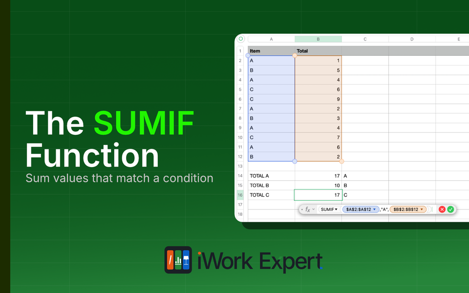
Let's say you run a small concession stand and want to know how much you made from Coke sales specifically, not Pepsi, not 7-Up, not any other soda. Just Coke. Adding up the whole sales column won't get you there, and picking out the Coke rows by hand gets old fast once you've got more than a handful of entries. What you need is a way to sum based on a condition. That's exactly what SUMIF does.
SUMIF adds up values in a range, but only for the cells that match a condition you set. The function name says it all: sum, if a condition is met.
SUMIF Function Details

Purpose: Returns the sum of the cells in a collection that satisfy a given condition you specify
Result: A sum of the matching cells
Syntax: =SUMIF(test-values, condition, sum-values)
Arguments: test-values, condition, sum-values (optional)
- test-values: the group of cells you're checking the condition against
- condition: the criteria each cell is tested against, which resolves to true or false. The condition is written as an expression, and your criteria can be expressed in a few ways:
- comparison operators (
=,<,>,<=,>=,<>) - constants (values that don't change)
- references (a value from another cell)
- ampersand concatenation operator (combine the contents of conditions or cells like less than what's in cell A2, i.e.,
"<"&A2) - wildcards (?*~) or REGEX
- comparison operators (
- sum-values (optional): the group of cells you actually want to add up. Leave this out and SUMIF just sums the test-values instead
If you're coming from Excel, SUMIF syntax looks like this =SUMIF(range, criteria, [sum_range]. Conceptually, Numbers arguments are setup in the exact same way, just the labels used for syntax is different: test-values instead of range, condition instead of criteria, sum-values instead of [sum_range]. Same function, different names on the same three boxes.
Quotations
Quotations in the SUMIF formula can get confusing because some conditions need to be in quotes while others do not. Direct cell references do not need quotes. However, if you type text or a comparison operators in the formula, those must be wrapped in quotation marks. Here is a really simple, three-tiered approach:
- Direct Cell References (no quotes):
A2
(Numbers reads the data inside the cell automatically) - Text or Hardcoded Operators (use quotes):
"Pepsi",">50","<=2026" - Combining Operators with Cell Reference (partial quotes):
"<="&A2
(notice the comparison <= is in quotes, but the ampersand and cell reference A2 is not)
More Ways to Write the Condition
- Sum if equal to 10 →
"10" - Sum if greater than 100 →
">100" - Sum if less than or equal to 100 →
"<=100" - Sum if equal to "bob" →
"bob" - Sum if not equal to "bob" →
"<>bob" - Sum if cell starts with "ka" →
"ka*" - Sum if cell contains "ka" anywhere →
"*ka*" - Sum if cell starts with "ka" and has exactly one character after →
"ka?" - Sum if equal to what's in cell A1 →
A1(no quotes) - Sum if less than what's in cell A1 →
"<"&A1 - Sum if less than a specific date →
"<2/1/2026"
Same rule of thumb as other IF functions: almost everything goes in quotes except a direct cell reference. For the ampersand operator specifically, keep the cell reference outside the quotes, or Numbers reads it as the literal text "B2" instead of whatever value is sitting in that cell.
When You'd Actually Use SUMIF
SUMIF is for the moment you want a total that's filtered by one thing. Not "how much did we sell," but "how much did we sell of this one item, this one client, this one category."
A few situations where that comes up in practice:
- You're tracking expenses by category and want to know how much went to "airfare" without manually adding up every supply line by hand.
- You run a small shop and want total sales for a specific product, separate from everything else moving through the register.
- You're managing freelance invoices and want to see how much one particular client has paid you to date, out of a sheet that has every client mixed together.
The common thread is one condition, one number back. The moment the question becomes two conditions at once, like "how much did this client pay in March specifically," SUMIF can't get you there on its own. That's the cue to move to SUMIFS instead.
How to Use the SUMIF Function in Numbers
I'll show a brief step by step guide on how to use SUMIF for finding the total of item "Hat" in column A followed by an example.
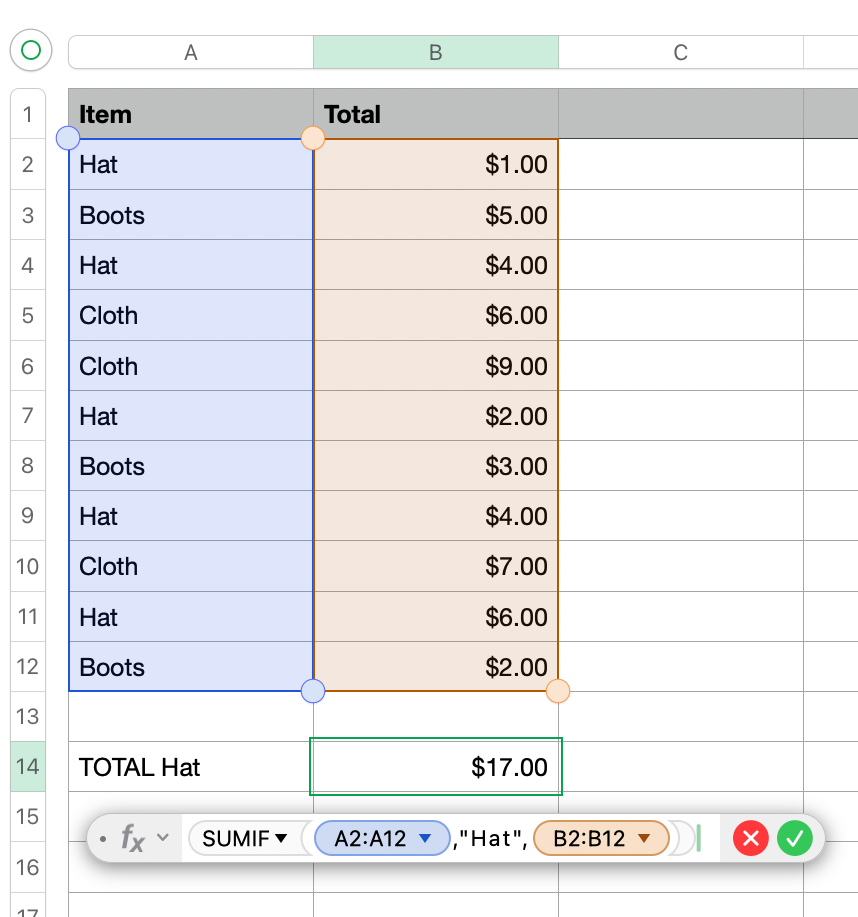
=SUMIF(A2:A12,"Hat",B2:B12) scans the Item column for matches and adds up the corresponding totals.Step 1: Reference the test-values The first argument is test-values. In our example, that's cells A2:A12.
Step 2: Enter the condition The second argument is condition. In our example, I want to sum only those items that are "Hat", so I'll enter "Hat". Note the quotation marks as this is a hardcoded text-operator.
Step 3: Reference the sum-values The last argument is sum-values. In our example, that's cells B2:B12.
Step 4: See the result The completed formula is =SUMIF(A2:A12, "Hat", B2:B12). This provides the result of $17.00 which is the total of cells B2 + B4 +B7 + B9 + B11.
An Example of Using SUMIF
Before reaching for SUMIF, double check you're actually only testing one condition. It's an easy thing to miss, since a request can sound simple and still be asking for two things at once.
Here's a common version of that trap: a salon owner asks, "Show me the total card payments for Luna." That sounds like one ask, but it's really two conditions: payment method (card) and stylist (Luna). SUMIF can't do that on its own. You'd need SUMIFS for that.
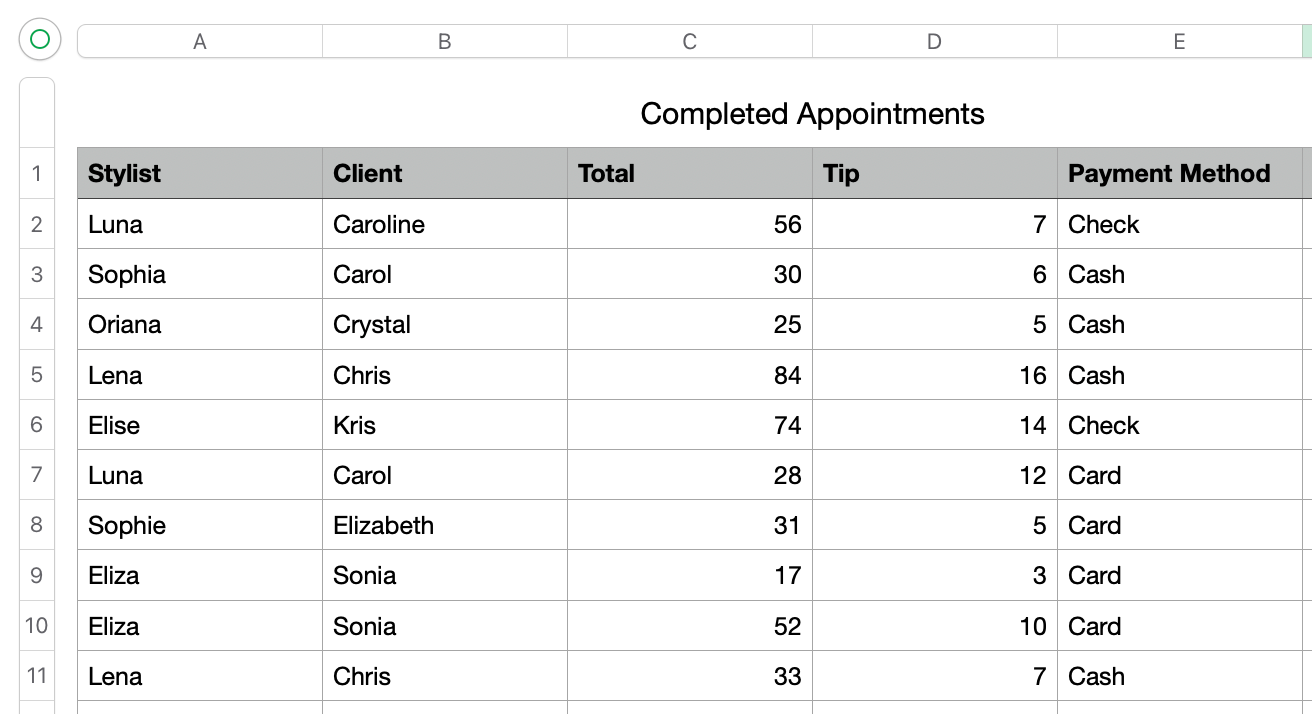
So let's stick with something SUMIF actually handles: totaling payments by stylist. Here's a simplified appointment log.
Total Payment to Each Stylist
- test-values: Column A (Stylist)
- condition:
"Luna" - sum-values: Column C (Payment)
- Formula:
=SUMIF(A2:A11,"Luna",C2:C11) - Result: $84 (rows 2 and 7: $56 + $28)
To answer other question variations, you're just pointing the same three arguments at different columns.
- Total Tips to Stylist "Luna": same test-values and condition, sum Column D (Tip) instead.
=SUMIF(A2:A11,"Luna",D2:D11)→ $19 - Total Payments by Client: test-values move to Column B (Client), condition becomes a client's name.
=SUMIF(B2:B11,"Carol.",C2:C11)→ $58 - Total Tips by Client "Carol": same as above, sum Column D instead.
=SUMIF(B2:B11,"Sarah K.",D2:D11)→ $18 - Total by Payment Method: test-values move to Column E (Method).
=SUMIF(E2:E11,"Card",C2:C11)→ $128, and=SUMIF(E2:E11,"Cash",C2:C11)→ $172
Same function, same structure every time. Only the columns change depending on what you're actually asking.
What SUMIF Isn't For
It's also worth pointing out what SUMIF isn't for. Picture that same salon appointment log. If the question is "how many appointments did Luna have this week" instead of "how much did Luna make this week," you're not summing anything anymore, you're counting rows. SUMIF will still run if you hand it that question, but it's built to total payment values, not tally how many rows matched. The fix is actually using the right function for the result you want: COUNTIF does the counting and skips the sum-values argument entirely, since there's nothing to add up.
The other direction shows occasionally for novice spreadsheet users. If there's no real condition, say you want the total of every payment in the log regardless of who did the work, writing a SUMIF condition that's built to match everything is solving a problem you don't have. The condition argument is the whole reason SUMIF exists; it's what decides which rows get included and which get skipped. If nothing actually needs filtering, SUM gets you the same total without having to use extra functions.
SUMIF Error Handling
The most common error comes from an argument range size mismatch. If test-values and sum-values have a range that is different numbers of cells (i.e., test-values range from A2:A10, but sum-values range from B2:B11) Numbers won't run the calculation. You'll see a red warning triangle on the cell, and clicking it shows a message to the effect that the range arguments need to be the same size. The fix is to recheck that both ranges start and end on the same rows.
A second, sneakier issue: the formula runs fine but returns 0 instead of erroring out. This usually means the condition isn't actually matching anything. Often, this is due to a column formatted as numbers instead of text or the condition text doesn't exactly match what's in the cells (extra spaces, a typo, mismatched capitalization on something that actually does need an exact match elsewhere in the formula chain).
If there is anything I've learned from spreadsheets, it's that you want to check your result for reasonableness. If you're getting a result but it looks wrong rather than an outright error, double check sum-values is pointing at the column you actually meant to total. It's an easy swap to make by accident, especially once a sheet has several similarly named columns.
Why Not Just Filter Instead?
For a one-off question on a small table, filtering works fine. Filter by stylist, jot down the total, clear the filter, repeat for the next stylist.
It stops being fine once the table grows. Picture that same appointment log six months from now, with hundreds of rows instead of ten. Filtering, reading off a total, clearing the filter, and doing it again for every stylist and every payment method turns into a lot of repetitive clicking, and you'd have to redo the whole thing every time a new appointment gets added. A SUMIF formula just sits there and updates itself the moment new rows come in.
Considerations and Limitations
These are some consideration and limitations when using the SUMIF function.
Considerations
- Sum-values needs to cover the same number of cells as test-values. If test-values spans 10 rows, sum-values needs to span those same 10 rows, or the total will be off (or the formula will error out).
- Avoid building the test-values range itself out of concatenation. Concatenation is fine inside the condition, just not the range you're testing against.
- If you're selecting multiple columns or rows for test-values, keep the range of cells consistent across each one.
- Cell references go without quotes. Just about everything else does.
Limitations
- SUMIF only checks one condition. For more than one, use SUMIFS.
- SUMIF isn't case sensitive. "card," "Card," and "CARD" are all the same.
SUMIF is the function to reach for any time you need a total filtered by one condition: sales for a specific item, payments to a specific person, totals by category. Once the three part structure (test-values, condition, sum-values) clicks, adapting it to a new question is mostly just swapping which columns you're pointing at.
If you find yourself needing to check two conditions at once, that's your cue to move on to SUMIFS.
For more detail, see Apple's support guide for SUMIF.
Related Functions
AVERAGEIF - returns an average of the matching cells that meet a single condition.
AVERAGEIFS - returns an average of the matching cells that meet multiple conditions at once.
SUMIFS - sums cells that meet two or more condition
SUM - adds up every value in a range, no conditions involved



Member discussion